RECURRENT NEURAL NETWORKS IN DEEP LEARNING/PYTHON/ARTIFICIAL INTELLIGENCE

Recurrent Neural Networks

• Backpropagation Through Time (BPTT) and Gradient Challenges
• Types of RNN and Architecture Variants
• Training and Working of RNN
• Advantages and Disadvantages of RNN

Artifical Recurrent Neural Networks (RNN) is a type of mn neural network that uses the output of the previous step as input to the current step. They are very efficient for sequential data types such as text and time series data. RNNs are designed to detect patterns in data sequences, including spoken word, text, genomes, handwriting, and numerical time series from various sources such as government agencies, stock markets, and sensors. They are integrated with popular apps like Google Translate, Siri, and Voice Search.

backpropagation in mn

A fundamental aspect of RNNs is their Hidden State, which retains information about a sequence, effectively acting as a memory state by recalling previous inputs to the network. RNNs use the same parameters for every input, performing consistent operations across all inputs and hidden layers to generate output. This parameter sharing reduces complexity in comparison to other neural networks. The output of an RNN is influenced by prior elements within the sequence. Additionally, parameter sharing across layers is a distinctive feature setting RNNs apart from other neural network architectures.

Image source original

The backpropagation through time (BPTT) technique is used by recurrent neural networks (RNNs). It differs slightly from regular backpropagation because it is designed for sequential data. The fundamental ideas of classical backpropagation are shared by BPTT: model training is accomplished by computing errors from the output layer toward the input layer, which allows for model parameter modifications. But a crucial distinction is that, in contrast to feedforward networks, which do not need error summation because there is no layer-to-layer parameter sharing, BPTT sums errors at each time step.

RNNs often encounter issues termed exploding and vanishing gradients, both related to the gradient's magnitude, which denotes the slope of the loss function along the error curve. Vanishing gradients occur when gradients become extremely small, leading to their continuous reduction until they approach insignificance (zero), halting learning. Conversely, exploding gradients manifest when gradients become exceedingly large, causing unstable model behavior and weight parameters reaching NaN representations. To mitigate these challenges, reducing the number of hidden layers within the neural network is a potential solution, alleviating some complexity inherent in RNN models.

Real-World Example for Recurrent Neural Networks

Let’s look at a real-world example for Recurrent Neural Networks, we have a startup that wants to revolutionize language learning. Our new product aims to provide personalized and interactive language education experiences to users worldwide. However, our startup faces a significant hurdle: to understand and predict users’ learning patterns to effectively tailor the learning experience.

To overcome this challenge, our startup looks at Recurrent Neural Networks (RNNs). These powerful AI models were trained on vast datasets of language learners’ interactions, including text inputs, audio recordings, and user engagement metrics. The RNNs can retain the memory of past inputs making them ideal for capturing sequential data, like the progression of a user’s language learning journey over time.

If a user interacts with our learning platform, then their interaction with our system is feed to our RNN model, which then analyzes the user sequence of inputs and detects the patterns or trends in the user-generated data. Our model can detect the learning pattern in the user's behavior by analyzing user-generated data, like their preferred learning topics, study behaviors, and areas where the user faces difficulties, our RNN model can adapt to the learning patterns in real-time which suit every user's learning behavior.

With the assistance of RNNs our learning platform transformed into a dynamic and personalized language platform. In our learning platform users can receive lesson recommendations, it has practice exercises, and our learning platform has its own feedback-based learning trajectory for its users which helps the user to learn a new language more effectively and make it more engaging.

How does RNN differ from a Feedforward Neural Network?

An Artificial Neural Network (ANN) is a type of Neural Network that is also known as a feedforward neural network because it does not have looping nodes. In this neural network-type model the information moves from the input node to hidden nodes and then the output node. It is a unidirectional neural network model. It is also known as a multi-layer neural network.

For applications where the input and output are independent, such as picture classification, feedforward neural networks are appropriate. They are unable to automatically remember data from prior inputs, though. They are less useful for examining sequential data because of this constraint.

Image source original

Recurrent Neuron and RNN Unfolding

A recurrent neural network's basic processing unit isn't referred to as a "Recurrent Neuron." The capacity to remain hidden is one of this unit's unique characteristics. This feature keeps information from prior inputs while processing, enabling the network to grasp sequential dependencies. The ability of the RNN to handle long-term dependencies is improved by variations such as Gated Recurrent Unit (GRU) and Long Short-Term Memory (LSTM) versions.

Image source original

Types Of RNN

There are four types of RNNs based on the number of inputs and outputs in the network they are: 

1. One to One
2. One to Many
3. Many to One
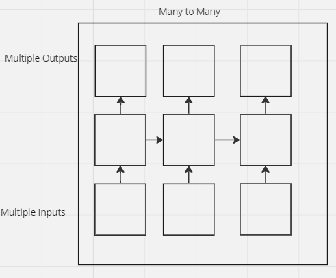
4. Many to Many

One-to-One: This type of recurrent neural network is often called a basic RNN or vanilla neural network because it works just like a simple neural network. This configuration has only one input and one output.

. 

Image source original

One to Many: as the name suggests in this type of RNN model there is one input signal and many output signals associated with it. It is very extensively used in image captioning in which a given image is used to predict a sentence having many words.

Image source original

Many-to-One: It is essentially the one-to-many type paradigm in reverse; in this model, numerous inputs are sent to the network at various network states, and each input produces a single output. We apply this kind of network to sentiment analysis tasks. When solving problems involving mn for sentimental analysis, we provide several words as input and anticipate the sentence's sentiment as the only outcome.

Image source original

Many to Many: Depending on the issue, this kind of neural network has a large number of inputs and outputs. One such issue type that uses many to many RNNs is language translation, where we give it several words in one language as input and it predicts many words in the other language as an output. 

Image source original

Recurrent Neural Network Architecture

The input and output structure of RNNs is similar to that of other mn in deep learning neural networks. However the way information moves from the input layer to the output layer is different. In RNNs, the same weights are maintained throughout the network, unlike deep neural networks where there are separate weight matrices for each dense network. 

Image source original

Variant RNN architectures

Bidirectional Recurrent Neural Networks (BRNN) represent a distinct variation within RNN architecture compared to unidirectional RNNs. While traditional RNNs rely solely on past inputs to make predictions, BRNNs incorporate future data, enhancing predictive accuracy. For example, in the phrase "feeling under the weather," the model can anticipate "under" as the second word more effectively by considering "weather" as the last word in the sequence.

Long-term memory (LSTM) networks, a widely used RNN architecture, effectively solve problems such as the vanishing gradient problem and long-term dependencies. LSTMs introduced by Hochreiter and Schmidhuber contain cells in hidden layers that contain three gates: an input gate, an output gate, and a forget gate. These gates play a vital role in controlling the flow of information needed to make accurate predictions. In situations where the information relevant to the prediction lies below, LSTMs allow the network to retain and use this distant context, which is crucial for tasks such as understanding a person's nut allergy in multiple sentences.

about mn

Similar to LSTMs, Gated Recurrent Units (GRUs) address short-term memory limitations commonly encountered in traditional RNNs. However, unlike LSTMs, GRUs do not rely on special "cell spaces"; Instead, they use hidden modes and integrate two ports: a reset port and an upgrade port. These gates control the amount and nature of the data stored in the network, providing flexibility in learning sequential data while maintaining computational simplicity compared to LSTMs.

How does RNN work?

The recurrent neural network (RNN) is undoubtedly made up of several fixed or constant activation function units, usually one for every time step. Every unit preserves what is known as its "hidden state," which is its internal condition. Usually, the network's stored knowledge or information up to a particular time step is contained in this concealed state. This hidden state changes at every time step as the RNN analyzes sequential data, representing the network's changing comprehension or recollection of the past.

The update of the hidden state in an RNN can be represented using a recurrence relation or formula that defines how this hidden state evolves across time steps. The recurrence relation expresses the change or update in the hidden state based on the current input, previous hidden state, and possibly other parameters or inputs related to the network's architecture and task at hand. This recurrent formula dictates how the network retains and updates its memory or knowledge as it processes sequential data.:

The formula for calculating the current state:

Here,

• h_t→current state (h subscript t)
• h_(t-1)→ previous state (h subscript (t-1))
• x_t→ input state (x subscript t)

The formula for applying activation function (tanh)

Here, 

• W_hh→ weight at the recurrent neuron (W subscript hh)
• W_xh→ weight at input neuron (W subscript xh)

The Formula for calculating output:

• y_t→ output (y subscript t)
• W_hy→ weight at the output layer (W subscript hy)

Backpropagation is used to update each of these parameters. Since RNNs process sequential data, we employ updated backpropagation, sometimes referred to as backpropagation across time.

Backpropagation Through Time (BPTT)

Since the RNN is an ordered neural network, each variable is computed individually in the predetermined sequence, such as h1 coming first, h2 coming next, h3 coming last, and so on. Consequently, we sequentially apply backpropagation to each of these hidden temporal stages.

Image source original

In the above diagram the 

• L(θ) (loss function) depends on h3
• h3 in turn depends on h2 and W
• h2 in turn depends on h1 and W
• h1 in turn depends on h0 and W
• where h0 is a constant starting state.

To better understand the above equation, we will apply backpropagation on only one row.

We also know how to compute this because it is the same as any simple deep neural network backpropagation.

We can also see how to apply the backpropagation to this term 

Because we already know h3 = σ(Wh2+b)

In a network like this which is in ordered form, we can’t compute 

 by simply treating h3 as a constant because it is also dependent on the W. The total derivative  has two parts:

• Explicit:  it treats all the other inputs as a constant.
• Implicit: it sums over all indirect paths from h_3 (h subscript 3) to W

Let's see how to achieve this

For better understanding, we short-circuit some of the paths and get this below equation.

After further modifying the above equation, we get the below equation

Where

Therefore, 

This algorithm is called backpropagation through time (BPTT) as we backpropagate over all previous time steps.

Training through RNN

The network receives a single-time step input and uses both the current input and the previous state to calculate the current state. This current state then becomes the previous state for the next time step, and this process is repeated for several steps, allowing the network to assimilate information from all previous states. After all time steps are completed, the final flow state is used to calculate the output. The output is compared to the target output, resulting in an error. This error then propagates back through the network and updates the weights. The RNN is trained over time using a back-propagation method that adjusts the network parameters based on the calculated error.

Advantages of RNN

Sequential Modeling: We use RNNs mainly with sequential data, we use RNNs with sequential data because RNNs can store and use previous memory or information processed. This feature is very useful when we are dealing with time series forecasting, language translation or speech recognition, or AI voice assistance. 

Variable-Length Inputs: Unlike traditional feedforward networks, RNNs can handle variable-length sequences. They process input sequences of varying lengths by sharing parameters across different time steps, allowing flexibility in handling diverse data formats.

Memory and Context Retention: RNNs possess memory cells that maintain information over time, enabling the network to capture long-term dependencies. This feature helps in learning and retaining context, crucial in tasks where understanding context is essential, like language translation or sentiment analysis.

Flexibility in inputs and outputs: RNNs can process inputs and produce outputs of various data types (e.g., sequences, vectors, or even structural data). This flexibility allows them to perform diverse tasks, including sequence generation, sentiment analysis, and mn machine learning translation.

Transfer Learning and Pretrained Models: - Already trained RNN models or embeddings learned model on large text dataset can take benefit of the downstream tasks, that can take advantage of transfer learning and can also reduce the need for extensive labeled data.

Adjusting to real-time data: RNNs can handle real-time generated data and it can also perform computations tasks on this data, which makes RNNs suitable for works like online prediction, video analysis, and live speech recognition.

Disadvantages of RNN

Vanishing/Exploding Gradient Problem: Because of vanishing or exploding gradients, RNNs may have trouble training over lengthy sequences. This happens when gradients propagate across time during backpropagation and either become exceedingly small (vanishing) or excessively large (exploding), making it difficult to understand long-range dependencies.

Difficulty in capturing long-term dependencies: despite their ability to retain information across time steps, standard RNNs can struggle with capturing long-term dependencies effectively. This limitation arises because the network might forget or misinterpret crucial information from distant past inputs when processing lengthy sequences.

Limited Short-term Memory: Traditional RNNs possess limitations in their short-term memory capacity. They might face challenges in retaining information for an extended duration, which can impact tasks where immediate context plays a significant role.

Computationally inefficient: RNNs present significant computational challenges, especially when dealing with long sequences. The inherent order of processing limits parallelism, resulting in slower training and inference time compared to feedforward networks.

Sensitivity to Hyperparameters: RNNs are sensitive to hyperparameters like learning rate, network architecture, and initialization. Selecting appropriate hyperparameters can be challenging, and improper choices might hinder their learning capability.

Training Instability: training RNNs can be unstable, especially when dealing with non-stationary data or noisy sequences. The network might have difficulties in converging or might be sensitive to data preprocessing.

Summary

Recurrent Neural Networks (RNNs) are an important architecture in the area of sequential data analysis. The RNN networks are developed in such a way that they can adapt during the processing of sequential data they can achieve this because they can store the data or memory from their previous steps, which helps them to do tasks like language processing, time series forecasting, and speech recognition easily. The RNN's ability to model temporal dependencies within sequences, helps it to make predictions based on previous data or inputs. RNN may have data storage as an advantage but it can face challenges like vanishing or exploding gradients during training, which can affect the RNN's ability to capture and leverage long-term dependencies. Additionally, they might face limitations in retaining short-term memory over extended sequences, impacting their understanding of immediate context.

To handle this limitation of RNN, it improved itself by adding variants like long-term short-term memory (LSTM), repetitive units (GRU), and attentional mechanisms. These techniques help the RNN to improve its ability which can help the RNN to handle or understand sequential data more easily and also help it to solve other problems like vanishing gradient problems, and capture long-term dependencies more effectively. Despite ongoing challenges, RNNs remain important for sequential data analysis, providing valuable insights and capabilities for tasks involving the understanding and processing of sequential data.

Python Code