PYTHON NUMPY

Python NumPy

Introduction

• Core Concepts of NumPy
• Advantages of NumPy
• Disadvantages of NumPy
• Best Practices for Using NumPy

One of the most powerful Python utilities is NumPy. It is a key Python module for scientific computing. This Python library provides a multidimensional array object, derived objects like masked arrays and matrices, and quick array operations like sorting, selecting, I/O, discrete Fourier transforms, basic linear algebra, basic statistical operations, random simulation, and more. NumPy works well with SciPy, Matplotlib, and pandas, which are used in scientific computing and data analysis, in addition to its speed. Since several libraries are compatible, users may solve complex issues by combining their capabilities. Overall, NumPy is essential for numerical computations and huge dataset processing in scientific computing, data analysis, and machine learning. Its performance, versatility, and integration possibilities make it essential to Python numerical computation. 

Essentially, NumPy is an ndarray object or array. Its n-dimensional data types are homogenous. NumPy supports huge, multidimensional arrays, matrices, and mathematical procedures to work with them. NumPy's array object, ndarray, lets users simply perform array operations.

The intrinsic C code of NumPy arrays speeds up operations compared to Python lists. NumPy also uses vectorized operations, which apply mathematical operations to arrays rather than individual elements, improving performance. NumPy is ideal for large datasets or complex mathematical tasks that require efficiency.

NumPy works well with SciPy, Matplotlib, and pandas, which are used in scientific computing and data analysis, in addition to its speed. Since several libraries are compatible, users may solve complex issues by combining their capabilities. Overall, Importing NumPy is essential for numerical computations and huge dataset processing in scientific computing, data analysis, and machine learning. It is essential to the Python numerical computing environment because of its performance, versatility, and integration possibilities.

NumPy

NumPy relies on the ndarray object. Its focus is the homogenous multidimensional array. In this table of numbers, all items are of the same type and indexed by a non-negative integer tuple. Importing NumPy dimensions name them axes.

The open-source Python library NumPy is utilized in practically every research and engineering sector. NumPy is the foundation of the scientific Python and PyData ecosystem and a global standard for numerical data in Python. Pandas, SciPy, Matplotlib, Scikit-learn, etc. utilize NumPy API extensively.

NumPy supports multidimensional arrays and matrices. NumPy has an ndarray with homogenous data in n dimensions and efficient techniques to work on it. NumPy can do many array math operations. 

Installing NumPy

First, we need to install the Python programming language to install the NumPy in our system. If we already have Python installed in our system then we only need to write one line of code to install Python. It can be any one of these two lines:

conda install numpy

OR

pip install numpy

This code may be typed in Python IDE or the system command prompt. Anaconda can install Python if the system does not already have it. The easiest method to learn Python is via Anaconda. Anaconda is great since it already has NumPy and other necessary packages, so we can use it for data analysis and other operations without much hassle.

Importing the NumPy

If we want to use NumPy and its function in our program in Python then first we need to import the NumPy package using the below written code.

import numpy as np

For clarity, we utilize NumPy's alias np in the above code. The preceding code is frequently used to import NumPy, and the alias is also an unofficial short name, thus we advocate using “np” as the single alias.

Real-World Example of NumPy Usage

Let's suppose we are working on a project that analyzes satellite images to monitor deforestation in a remote rainforest. Python’s NumPy and pandas library in Python prove indispensable in handling vast amounts of data efficiently.

We start with importing the NumPy library and loading satellite images into NumPyPython arrays. These arrays represent pixel values, with every pixel containing information about color intensity or reflectance.

With NumPy, we can perform various operations on these data/arrays. For example, we use NumPy’s slicing and indexing capabilities to extract specific regions of interest from the images, like areas with significant tree cover loss.

Next, we can apply mathematical operations provided by NumPy to manipulate pixel values. For instance, we might calculate the difference between images taken at different time points to detect changes in forest cover over time. NumPy’s broadcasting feature allows us to perform these operations efficiently across entire arrays.

If we want then we can also leverage NumPy’s statistical functions to analyze image data. We compute summary statistics like mean, median, and standard deviation to quantify deforestation rates and assess the severity of environmental degradation.

Furthermore, we can also use NumPy to facilitate image processing tasks like filtering and smoothing. We can apply convolution operations using NumPy’s convolve function to enhance image clarity and remove noise, improving the accuracy of our deforestation detection algorithm.

Finally, NumPy integrates seamlessly with other Python libraries like Matplotlib and OpenCV for visualization and further analysis. We use Matplotlib to create visualizations of deforestation patterns and OpenCV for advanced image processing tasks like edge detection.

In the above example, we learn that the NumPy library empowers us to efficiently process, analyze, and visualize satellite imagery, enabling crucial monitoring and conservation efforts in environmentally sensitive areas.

Difference between a Python list and a NumPy array 

In contrast to lists, NumPy offers several fast and efficient techniques for generating arrays and working with numerical data. However, Python lists can include many data types, while numpy arrays should be homogenous. NumPy employs homogeneous elements because non-homogeneous data is hard to manipulate mathematically.

Why do we use NumPy?

NumPy is quicker and smaller than Python lists, therefore we utilize it. The arrays are easy to use and utilize less memory. Since arrays consume less memory, NumPy stores data in less memory and defines data types. Our codes may be optimized further.

What is an array?

NumPy's fundamental data structure is an array. A grid of values with raw data, element position, and element interpretation properties is an array. The grid of array elements can be indexed in several ways. All elements are of the same type, called the array dtype.

We can index an array using a tuple of nonnegative integers, Boolean, another array, or integers. Array rank indicates dimensionality. NumPy's shape function determines array size and dimensions. Let's examine the 2-D array form code. 

The above code outputs (2,5), indicating the array's form and size. 2 is its dimensions and 5 is its array size.

Nested lists can be used to establish a NumPy array for two- or more-dimensional data, as seen in the preceding code. Look at a higher-dimensional NumPy array containing lists and try to access its elements. 

In the given code, square brackets are used to access array items or lists. Before accessing any NumPy element, understand that its index starts with 0. It means that to access the first element (in this case the list) of our array, we must access element 0 as shown in the above code, and to access any item from the list, we must pass the index of the value of the list, a comma, and the index number of the item we need to access (which starts with 0).

More information about arrays

Sometimes "ndarray," short for "N-dimensional array," is used to describe an array. N-dimensional arrays are any number of dimensions. Arrays of one dimension, two dimensions, and so on can also be stated. The NumPy ndarray class represents vectors and matrices. A matrix is a two-dimensional array, while a vector is one-dimensional (row and column vectors are the same). Many use "tensor" to refer to 3-D or higher-dimensional arrays. 

What are the attributes of an array?

A fixed-size array holds equally sized and typed items. The shape determines the array size and objects. An array is shaped by a tuple of non-negative integers defining dimension widths.

Axes are NumPy dimensions. A 2D array might look like this: 

The above array contains two axes: 2 (rows) and 3 (columns).

Like other Python container objects, indexing or slicing an array lets one manipulate its contents. Unlike ordinary container objects, arrays may share data, thus changes to one may affect another.

The qualities of an array represent its intrinsic data. You can often access an array's attributes to get or update its characteristics without creating a new array.

How to create a basic array

Creating an array in Python using NumPy is simple—use “np.array()”. NumPy requires a list to generate a basic array. We may also select our list's data type.

A numpy.dtype data type object specifies how to interpret the bytes in the fixed-size block of memory that corresponds to an array item. The type describes the following data aspects:

• It describes the type of the data (integer, float, Python object, etc.)
• It is also able to describe the size of the data (how many bytes are in e.g. the integer)
• Byte order of the data (little-endian or big-endian)
• An aggregate of different data types, such as one that describes an array item made up of an integer and a float, if the data type is structured
• What are the names of the structure's "fields" and the methods for accessing them?
• What is the data type of each field, and
• Part of the memory block each field takes.
• If the data type is a sub-array, what is its shape and data type.

Let's create a simple array using NumPy in Python: 

The above code array can be visualized in the below diagram.

These image simplify NumPy mechanics and ideas to help you understand them. Arrays and their functionalities are more complex than shown here!

Image source original

NumPy lets us generate an array with all 0s or 1s as well as a succession of items. Check out the Python code for producing them:

NumPy can build empty arrays. The method empty produces a random array based on the memory situation. Use empty over zeros or similar for speed; fill every element thereafter!

If we want we can create an array with a range of elements. Let’s look at the code: 

If we need we can create an array with a range of intervals that are uniformly spaced. You will need to provide the step size, and the first and last numbers to accomplish this.

We can also use NumPy’s linspace() function to create an array whose values are spaced linearly in a specified interval. Let’s look at its code:

Adding, removing, and sorting elements

NumPy's sort(), concatenate(), and other methods let us add, delete, and sort Python arrays. Using “np.sort()” to sort a NumPy array element is easy. Every time we call the function, we may give axis, kind, and order.

Let’s create an array using Python and sort it using the NumPy function. 

In the preceding code, we first build an unsorted NumPy array. After constructing the array, use NumPy's sort function to sort it by passing it to the array.

Other sorting functions can be used for different sorts. Let's examine and write their codes to comprehend.

argsort -  Use the kind keyword-defined algorithm to sort indirectly along the axis. It produces a sorted array of indices with the same form as that index data along the provided axis. Its syntax:

numpy.argosrt(a, axis=-1, kind=None, order=None)

let’s look at its Python code:

For a two-dimensional array let’s see the code and its output 

lexsort – Key sequences accomplish indirect stable sorting. Lexsort generates an array of integer indices that indicate the sort order of many columns given multiple sorting keys, like spreadsheet columns. The last key in the sequence determines the main sort order, the next-to-last key determines the secondary sort order, etc. The main argument must be a succession of things that can be turned into arrays of the same shape. If the keys parameter is a 2D array, the rows are the sorting keys, and the last row, second last row, etc. are sorted. Look at its syntax and one code example:

numpy.lexsort(keys, axis=-1)

searchsorted – Finds indexes for inserting elements to maintain order. Determine the indices into a sorted array ‘a’ so that the order of ‘a’ would be intact if the appropriate components in ‘v’ were inserted before the indices.

Let’s look at an example where ‘a’ is sorted:

Side	Returned index i satisfies
Left	a[i-1] < v <= a[i]
Right	a[i-1] <= v < a[i]

Let’s look at Python code for better understanding:

partition – A partitioned array is returned. It copies the array and rearranges its items so that the value at location k is as in a sorted array. Every element before the kth element is less than or equal to it, while every element after it is greater. The components of the two divisions are not ordered.

Let's examine partition syntax and sample code with an explanation.

Numpy.partition(a, kth, axis=-1, kind=’introselect’, order=None)

In the preceding code, we define the kth element as 4 and output p[4] as 2; all items in p[:4] are less than or equal to p[4], and all elements in p[5:] are greater. Therefore, the split might look like this for clarity:

[0, 1, 2, 1], [2], [5, 2, 3, 3, 6, 7, 7, 7, 7]

We may use concatenate() to add two or more arrays together as well as sort them. This function concatenates arrays along an axis. Look at its syntax and explain it to comprehend.

numpy.concatenate((a1, a2, …), axis=0, out=None, dtype=None, casting=”same_kind”)

The preceding code uses array_like parameters a1, a2,... Arrays must have the same form except for the axis dimension (always the first).

axis: int, optional—the array-linking axis. Flatten arrays before use if the axis is None. By default, it is 0.

out: If provided, ndarray will be the outcome's location. Shape must match what concatenate would have generated without an out argument.

dtype: If specified, the target array will contain this dtype. Unavailable without.

casting: {‘no’, ‘equiv’, ‘safe’, ‘same_kind’, ‘unsafe’} (optional) - controls data casting type. It defaults to ‘same_kind’.

After understanding the syntax, let's examine how it works with different values 

In NumPy, we can remove elements from an array using various functions such as ‘numpy.delete()’ or Boolean indexing. Let’s look at these different methods:

Using numpy.delete() – this function removes elements along a specified axis from an array. The ‘numpy.delete()’ function takes three main arguments:

• Input array (‘arr’): this is the array from which we want to remove elements. It’s the original grid of values that we’re working with.
• Indices to remove (‘obj’) : these are the positions of the elements you want to remove along the specified axis. It could be a single index, a list of indices, or even a slice.
• Axis (‘axis’) : this specifies the axis along which the deletion will occur. If we don’t specify an axis, it will default to removing elements along a flattened version of the array.

Syntax of numpy.delete() function: - numpy.delete(arr,obj, axis=None)

Using Boolean indexing: we may filter elements by condition. To comprehend the image, we want to choose elements from a NumPy array of values that fulfill particular criteria. Here comes Boolean indexing. Instead of defining explicit indices, Boolean indexing lets us define a mask—an array of True or False values—to indicate which elements meet our constraints. Three phases comprise this process: -

First, we define a condition that evaluates to True or False for each array entry. This condition might be anything from simple comparisons (greater than, less than) to complicated logical processes.

NumPy applies the condition element-wise to the original array to create a mask. We receive a Boolean mask with each member representing whether the original array element's criteria are True or False.

Final Boolean indexing: We choose elements from the original array using this mask. NumPy filters out items other than those with True mask values by bypassing the mask as an index.

This method is flexible and efficient for data manipulation. We may dynamically choose components using basic to complicated criteria. Boolean indexing simplifies NumPy array manipulation and data analysis workflows by cleaning data, extracting features, and executing conditional actions.

Let’s look at the syntax for it and a code example:

Syntax - Array[‘condition’]

How do you know the shape and size of an array?

‘ndarray.ndim’ The NumPy property ndarray.ndim shows the number of dimensions in an array. Creating a NumPy array creates a data structure. This structure can be arranged in various ways. Consider a two-dimensional array a grid or table, a one-dimensional array a list of values, etc. This structure deepens with each level.

The number of dimensions in our array is shown by ‘ndarray.ndim’. An array with one dimension has a ‘ndim’ value of 1. ‘ndim’ is 2 for a two-dimensional array like a matrix and higher for higher dimensions.

Understanding the number of dimensions affects how you can access and use array data. You'll use different ways to index a 2D array vs a 3D array.

Basically, ndarray.ndim makes it easy to see your array's structure and dimensions. This is essential for utilizing NumPy arrays in arithmetic and computing.

ndarray.size shows the number of elements in our array. The array shape's elements produce this. Building a NumPy array organizes data into a structure. This format might be a matrix, array, or list. Whether the array is large or small, ndarray.size counts every element.

A one-dimensional array has the same size as its elements. It is the total number of elements in all two-dimensional array rows and columns. Higher-dimensional arrays include all-dimensional items.

It's important to know an array's size since it reveals its data capacity. This data helps manage array memory by estimating its utilization. Knowing the size lets the user efficiently cycle through the array and calculate or analyze its components.

To conclude, ndarray.size quickly determines the number of items in a NumPy array, which is vital for rapidly manipulating, analyzing, and using arrays in numerical computation.

ndarray.shape displays a tuple of numbers indicating the number of entries in each array dimension. The form of a 2D array with 2 rows and 3 columns is (2, 3).

NumPy arrays can take several forms depending on how our data is structured. Ndarray.shape shows how big each array dimension is.

If the array were one-dimensional, its form would be a tuple with one value representing its length. Two-dimensional arrays, like matrices, are tuples with two values, representing rows and columns. Similar to higher-dimensional arrays, their forms include dimension sizes.

It's important to understand array form since it simplifies data structure. Indexing, slicing, and other array operations need knowledge of member axes.

To conclude, ndarray.shape simplifies NumPy array size for computational use.

Let's generate a 3-dimensional numpy array and apply each technique to examine the results.

In the above code, we can see all the output of these methods and we can also verify them with the description we provided for them that is they produce the correct output.

Can we reshape an array?

We can reshape numpy arrays with numpy.reshape(). The reshape() method reshapes the array without affecting its contents. We must remember that the reshaped array must contain the same number of elements as the original array. If we have an array with 12 elements, our reshaped array must likewise have 12 elements.

For a better understanding let’s create an array and reshape it using the reshape function.

We can use the reshape() function to reshape our array. We can reshape the above array to an array that has three rows and two columns:

With numpy.reshape(), we can provide a few optional parameters. They are provided in below code:

The code above specifies newshape as the new shape. You can specify an integer or tuple. Given an integer, the result will be an array of the specified length. The form should match the initial one.

F reads and writes items using a Fortran-like index order, while C uses a C-like index order. Fortran contiguous memory elements can be read/written in C-like order, otherwise, or in Fortran-like index order. (This argument is optional and not necessary.)

How to convert a 1D array into a 2D array (how to add a new axis to an array)

Numpy's newaxis and expand_dims functions may now expand arrays. Let's discuss each one individually.

Once applied, numpy.newaxis may add one dimension to our array. It means that using the "newaxis" function, we can make a 1D array 2D, a 2D array 3D, and so on. It may also place new axes.

The ‘newaxis’ function is handy for broadcasting arrays of varied dimensions or conducting actions that need certain array forms. It's a simple approach to restructure arrays without creating new ones, conserving memory and computing resources.

To put it simply, ‘newaxis’ expands NumPy array manipulation, making data manipulation more flexible and expressive. Whether we're working with basic arrays or large multi-dimensional data, ‘newaxis’ lets us reshape and change them.

For example, let’s look at the code to see how it changes the dimension of an array.

The preceding code sample uses np.newaxis to directly transform a 1D array into a row or column vector. Inserting a first-dimensional axis converts a 1D array to a row vector. Use the code to examine this:

The preceding code inserts the axis in the first dimension, giving row_vector a form of (1, 6) where 1 is a row and 6 is the number of columns.

Let's use Python code to transform the vector into a column vector as well as a row vector.

The preceding code inserts an axis in the second dimension, giving col_vector a shape of (6, 1), where 6 is the number of columns and 1 is the number of rows.

Expand_dims is another numpy function for increasing array dimensions. Inserting a new axis at a specific place expands an array. In NumPy arrays, ‘expand_dims’ may be used to change the geometry of an array for particular operations or needs. It increases the dimensionality of our array by adding dimensions.

For instance, we wish to convert a 1D array of integers into a 2D array with rows and columns for each number. Use ‘expand_dims’ to add a new axis in the desired direction.

The ‘expand_dims’ function takes two main arguments:

• ‘a’: the input array that we want to expand.
• ‘axis’: the position along which we want to insert the new axis. If not specified, the new axis is added at the end of the array’s shape.

The ‘axis’ argument lets us choose where to put the new axis, allowing us to customize our array.

In conclusion, ‘expand_dims’ makes array form adjustment easy for NumPy, making data manipulation for computational jobs easier. ‘expand_dims’ lets us reshape arrays to meet our needs, whether they're basic or multi-dimensional.

For a better understanding of the ‘expand_dims’ let’s look at the Python code:

In the preceding code, we construct an array using numpy and verify its form using the shape method. In the second code, we increase the array's dimensions using the "expand_dims" function and provide the array a with axis=1 (row). The shape method is used in the next line to show the array's 6 columns and 1 row. The following block of code uses the ‘expand_dims’ function again, but this time we pass axis=0 to expand the array rows. The output contains 1 column and 6 rows.

Indexing and slicing

Python arrays may be indexed and sliced like lists. Indexing in NumPy arrays allows accessing specific elements or subsets. Essential for data analysis and processing activities. Numerous indexing algorithms in NumPy allow users to efficiently retrieve data. Like Python lists, integer indices provide direct access to items in one-dimensional arrays. Indexing multi-dimensional arrays is harder since numerous axes must be defined. NumPy supports both basic and sophisticated indexing, which retrieves non-contiguous elements or creates views of the original array using arrays or tuples of indices. Knowing NumPy's indexing algorithms is crucial for accessing and manipulating data from arrays in numerical computing workloads.

Let’s look at different ways to index or slice an array using Python code:

For a better understanding of the above code, we can visualize it in the below diagram. 

Image source original

In the preceding code and picture, array slicing or indexing is similar to list indexing or slicing; it has negative indexes starting at 0 and going to n-1. It can also accept a colon for element access.

Slicing or indexing is necessary because we may wish to extract a segment or certain array members for analysis or other activities. For that, we must subset, slice, or index our arrays.

NumPy makes indexing or slicing arrays easy under certain situations. Look at the Python code:

We can also select numbers that are equal to or greater than a particular number. 

If we want, we can also do other operations as well like using division, AND (&) and OR (|) operators, etc. Let’s look at them one by one in code:

In the above code, we can see some of the different operations we can perform on the arrays.

The logical operators & and | can yield Boolean values indicating if an array's items meet conditions. This is useful for arrays with names or category values. Let's examine the code's Boolean output.

Numpy.nonzero() can pick items or indices from an array if we supply a conditional parameter in the bracket. Look at the code to understand.

Returning a tuple of arrays for each dimension. The first and second arrays represent the row and column indices, where the values are.

Zip the arrays, loop over the coordinates, and output the element positions if desired. Consider the demo Python code: 

If we want then we can also use np.nonzero() to print the elements in an array that are less than 5 with the below code (we use 5 because its code is already written above) 

The returned array of indices will be empty if the element you're seeking isn't in the array. For example let’s look at the Python code: 

How to create an array from existing data

We may generate an array from existing data using slicing and indexing, as well as numpy.vstack(), hstack(), hsplit(), view(), and copy(). Due to our knowledge of slicing and indexing, we just examine their code in this part and explore other approaches in depth.

In the above code we grabbed the section of our array/data from index position 3 through index position 8. (note it is n-1)

vstack - NumPy's ‘vstack’ method stacks arrays vertically to create a new array with extra rows. We can stack arrays on top of each other. It's useful to concatenate arrays with the same amount of columns to increase the dataset vertically. If we have two arrays with the same amount of features, we can stack their rows to produce a single array with ‘vstack’. This function simplifies data integration from several sources for processing and analysis by combining datasets or adding new observations to data arrays. Look at the Python code: 

In the above code, we can see that the ‘vstack’ method stacks two arrays into one vertical array.

hstack - The NumPy ‘hstack’ function may horizontally stack arrays along their horizontal axis to create a new array with extra columns. It allows side-by-side array concatenation. This method expands the dataset horizontally, making it useful for combining arrays with the same amount of rows. For instance, ‘hstack’ can combine two arrays with the same number of observations but representing different data sets into a single array with their columns close to each other. This function simplifies data integration from numerous sources for analysis or modification by joining datasets or adding new variables to data arrays. To better comprehend utilizing the aforementioned arrays, let's examine its Python code: 

As we can see ‘hstack’ horizontally stacks two or more arrays into one. 

hsplit - A NumPy method named ‘hsplit’ splits an array horizontally along its columns. This technique helps split large arrays by columns. When using ‘hsplit’, you may specify where to split the array or how many equally sized subarrays to create.

A 2D array representing a dataset might be divided into arrays with information on a subset of features, assuming each column represents a feature. Give ‘hsplit’ the number of sub-arrays or column indices to split.

This function simplifies splitting large datasets into smaller chunks for processing or analysis. It's especially useful when you need to divide computational tasks across many processors or nodes or apply different operations or analyses to certain data parts. Overall, ‘hsplit’ increases NumPy data processing task flexibility and efficacy. Let's examine the Python code to understand ‘hsplit’: 

The preceding code uses the reshape function to build a 12-element array for each row. To split the above array into three equal-sized arrays, run the following code: 

In the above code, we can see that we split the array ‘x’ into 3 equal parts by just passing the array ‘x’ and 3 as an argument in the ‘hsplit’.

If  we need then we can split our array after the third and fourth columns, we need to run the below code:  

In the above code, we pass the array ‘x’ as an argument and after that, we open a bracket and pass the column number we want to split as another argument and then close the bracket.

view – the ‘view’ function creates a new array object that appears like the original array (a shallow copy). A NumPy "view" lets you view array data without duplicating it. This is like several panes in a dataset. A view of an array is a new array object with custom indexing and reshaping characteristics but the same contents.

Views simplify data management and analysis by reducing memory allocation and data duplication. Instead of producing fresh arrays, establishing views with different sizes, lengths, or data types gives you greater data access and handling freedom.

It's important to realize that opinions might be unclear. Many NumPy operations return views instead of copies of the original data, which might cause unexpected behavior if not understood. Therefore, importing NumPy in Python memory management and data manipulation needs a knowledge of views.

Overall, machine learning NumPy views are a good method to interact with data, saving memory and resources while maintaining flexibility and usability in array operations.

A fundamental data science NumPy concept is viewed! Indexing and slicing return views when possible in NumPy. This is faster and consumes less memory because no data copy is needed. It's important to understand that view data alters the original array! See a code to comprehend the view: 

The preceding code gives variable ‘b1’ a view of array ‘a’'s first row. Because views share data, changing ‘b1’ changes ‘a’ too. Thus, altering ‘b1[0]’ to 99 turns ‘a[0, 0]’ to 99.

copy - NumPy's "copy" function creates a new array with the same contents but is independent of another. Cloned array modifications have no effect on the original array, and vice versa. Copies are useful for editing data without affecting it.

NumPy has two main array copying methods:

Shallow Copy: A shallow copy creates a new array object while preserving the old data. Although the arrays are different, data changes in the copied array affect the original array and vice versa.

Deep Copy: Deep copies make a second copy of the array's data and nested objects. The original array is unaffected by cloned array modifications, and vice versa. Deep copies ensure that changes to one array don't impact the other.

Knowing whether to utilize shallow or deep copies affects memory use and code behavior. Shallow copies are faster and use less memory, but changes to one array may affect the other. Deep copies are independent but consume more memory and are slower for large arrays.

In conclusion, NumPy's ability to duplicate arrays allows data manipulation without altering the original, making arrays safe for numerical computing experiments. 

Modifying the shallow copy ‘shallow_copy’ does not affect the array ‘a’. Because shallow copies share the same data as the original array, they construct a new array object. Thus, altering ‘shallow_copy’ only alters the copied array, leaving ‘a’ unchanged. 

Original array ‘a’ stays untouched after deep copy ‘deep_copy’ modification. Because a deep copy copies the array and its data, it is independent. Therefore, changing ‘deep_copy’ does not affect array ‘a’, and vice versa.

Basic array operations

This section covers addition, subtraction, multiplication, division, and more. After creating arrays, we may use them. If we build two arrays, we can add, subtract, divide, and multiply them using their signs.

NumPy array addition joins items from one or more arrays to create a new array with the same structure. It extends addition to any-dimensional arrays. When we combine two NumPy arrays, the NumPy array adds each element to its matching element in the second array. If we add two 1D arrays, [1, 2, 3] and [4, 5, 6], then we get [5, 7, 9] and when we add two 2D arrays element-wise then, the NumPy adds the matching elements from each array to create a new 2D array. NumPy broadcasts, allowing us to add different arrays with automatically aligned dimensions. Python's numerical calculation relies on addition, a powerful tool for data processing, and NumPy array math.

Subtraction in NumPy arrays involves removing the identical elements from two arrays to generate a new array with the same structure. Subtraction in fundamental arithmetic is extended to any-dimensional arrays using this approach. Subtracting two NumPy arrays element-wise means that we are subtracting each element from the other according to their elements. If we subtract two 1D arrays [3, 2, 1] and [1, 2, 3] then we get [2, 0, -2] array. If we subtracts two 2D arrays element-wise then it creates a new 2D array. NumPy's broadcasting function aligns array dimensions when subtracted. Python data management and mathematical calculations depend on NumPy array subtraction for many numerical computing tasks.

NumPy array division splits matching elements across two arrays to create a new array with the same structure. This operation lets arrays of any dimension employ division beyond ordinary arithmetic. Dividing two NumPy arrays element-wise divides each element by its corresponding element of the other array. If we divide two 1D arrays, [6, 12, 18] and [2, 4, 6], then we get [3, 3, 3] array. Divide two 2D arrays element-wise give us a new 2D array . Divide arrays of different forms using NumPy's broadcasting function, which aligns their dimensions. Division in NumPy arrays makes Python mathematical operations and data processing efficient for many numerical computing tasks.

NumPy arrays multiply two arrays by their elements to create a new array with the same structure. This procedure extends fundamental arithmetic multiplication to any-dimensional arrays. Each element in one NumPy array is multiplied by its matching element in the second array. Multiplying two 1D arrays [1, 2, 3] and [4, 5, 6] yields [4, 10, 18]. Multiplying two 2D arrays element by element creates a new 2D array with the same form. Multiplying arrays of different forms with NumPy's broadcasting function aligns their dimensions. NumPy array multiplication makes Python mathematical calculations and data processing efficient for many numerical computing tasks.

First, construct two arrays and do all the above actions on them. Image representations are shown.

Image source original

In the above diagram we can see that we have two arrays now in new diagrams we see the results when we apply the basic operations to it.

let’s see the resulting diagram for a better understanding.

Image source original

Let’s do more operations on the same two arrays. 

Image source original

The diagram and additional array operations are shown in the above programs.

Simple math is easy using NumPy. We may use sum() to get the sum of an array's items. It works with 1D, 2D, and higher-dimensional arrays.

Data analysis using Numpy

NumPy's sum() function calculates an array's axis sum. This versatile function lets us calculate the sum of each array member along a single axis, many axes, or both. If no axis is specified, sum() sums all array items. The function calculates the sum along an axis, collapsing the array along that dimension and creating a smaller array. This helps compute row or column sums in multidimensional arrays. The Python sum() function is essential for many numerical computations and data processing tasks due to its simple and effective manner of computing sums over arrays of arbitrary dimension.

Let’s look at the code for better understanding.

The preceding code builds a NumPy array ‘a’ with ‘[1, 2, 3, 4]’. Then, it uses the ‘sum()’ method to sum the array, returning ‘10’.

See the code below to sum the array over its axis. Row-wise addition is axis 0 while column-wise addition is axis 1.

In the following code, axis=0 adds row-wise, creating an array([3, 3]). Changing the axis=1 adds column-wise, creating an array([2, 4]).

Broadcasting

Sometimes we need to operate between an array and a number or two different-sized arrays. For instance, we may use an array and a number to convert miles to kilometers.

data analysis NumPy's broadcasting capability lets you join or operate on arrays of varied shapes. NumPy learning automatically broadcasts compatible arrays for element-wise operations between arrays, improving efficiency.

NumPy compares array shapes element by element in transmission, starting at the right (trailing dimensions) and advancing to the leading dimensions. If the dimensions are compatible—equal or one is 1, NumPy automatically expands the smaller array to match the bigger array along a dimension.

If we have a 1D array [1, 2, 3] and a scalar 2, NumPy will broadcast the scalar to be [2, 2, 2]. This replicates the scalar in other dimensions. We can efficiently perform element-wise operations like addition, subtraction, multiplication, and division.

Broadcasting aids in working with arrays of different forms without altering them. It streamlines and condenses code efficiently. Understanding broadcasting is essential to using NumPy for array manipulation and numerical processing.

Let’s look at Python code for better understanding. 

This example assigns 10 scalar values to each element of the 1D array a (3,). NumPy broadcasts the scalar value to match a to add 10 to each array element. Broadcasting simplifies NumPy element-wise operations between arrays and scalars.

Let’s look at a more complex example containing two arrays. 

Example: 2D array an is (2, 3) and 1D array b is (3,). NumPy automatically broadcasts the 1D array b to have the same form as an in the second dimension when we execute a + b. Thus, adding each element in b to its corresponding element in an adds [10, 20, 30] to each row of an. This shows how broadcasting simplifies NumPy element-wise operations over arrays of various types.

More useful array operations

This section covers maximum, minimum, total, mean, product, standard deviation, and more.

NumPy aggregates too. We can immediately run mean to obtain the average, prod to multiply the items, std to get the standard deviation, and more in addition to min, max, and total.

max() - NumPy's max() function finds the maximum value in an array or along an axis. Array NaN values are disregarded and the maximum element is returned. By default, if no axis is specified, the method returns the greatest flattened array value or overall dimension.

Another option is to identify the largest value on an axis. Set axis=0 to find the maximum value along rows and axis=1 to find it along columns in a two-dimensional array.

This function is useful for finding the greatest value in a dataset or extracting maximum values along certain axes. It quickly and efficiently finds the biggest objects in arrays of any size. 

• A 2D array of data is created.
• We use max() function when we want to get the maximum value of an array along it rows and columns.
• In the above codes' output we can see that the maximum value row-wise is ([4,5,6]) and the maximum value column wise is ([3,6]) and the maximum value in the all array is (6).

min() - The min() function of NumPy used to find the minimum value of an array or it axis wise. Min(), like max(), provides the flattened array's minimal value across all dimensions if no axis is given.

Another option is to identify the lowest value on an axis. Set axis=0 to find the least value along rows and axis=1 to find it along columns in a two-dimensional array.

This method is useful for finding the least value in a dataset or extracting minimum values along certain dimensions. It quickly finds the smallest objects in arrays of any size. 

This sample of code shows how to determine the minimum values in a 2D array called data using NumPy's min() function.

• The min_value = data.min() line determines the minimal value in the array. Since 1 is the smallest array element, it gets printed.
• The line min_row_values = data.min(axis=0) retrieves the minimal values for each column in the array rows. The minimum column values are [1, 2, 3].
• Using min_col_values = data.min(axis=1), the minimum values for each row are calculated along the array columns. The minimum values in each row are [1, 4].

All things considered, this code demonstrates how to effectively identify minimum values in arrays using NumPy's Python min() function, either throughout the array or along particular axes.

Sum() -  we already learned about the sum() function it works the same therefore we directly jump on the code.

• sum_total = data.sum() sums all the values in the array. The sum of all array items is displayed.
• Data = sum_row_values.sum(axis=0) finds the sum for each column along the array rows. The result shows column sums.
• Data = sum_col_values.sum(axis=1) finds the sum for each row along the array columns. The result shows row sums.

Overall, this code shows how to effectively compute sums in arrays along particular axes or over the entire array using NumPy's sum() function.

Let’s look at the diagram to visualize the operations.

Image source original

mean() - NumPy's mean() function calculates the array's arithmetic mean along a given axis or axes. NaN values in the array are disregarded and the average value is returned. If no axis is specified, the function computes the mean of all flattened array items to get the mean value across all dimensions.

Another option is to calculate the mean along an axis. Set axis=0 to compute the mean along rows and axis=1 to compute the mean along columns in a 2D array.

This function is useful for computing a dataset's average or extracting axes' mean values. It quickly and efficiently determines data central tendency in arrays of any dimension.

• data.mean() is use to calculate the mean of an array.
• data.mean(axis=0) - it is used to calculate the mean of the array along its rows it means that we calculate the mean of the row of the array.
• data.mean(axis=1) - it is used to calculate the mean of the array along its columns it means that we calculate the mean of the columns of the array.

Results are presented with mean values for the array, rows, and columns.

product() - NumPy's product() method calculates an array's product along a given axis or axes. NaN values are ignored and the array product is returned. The method defaults to finding the product of all flattened array items across all dimensions without an axis.

Another option is to calculate the product along an axis. In a two-dimensional array, axis=0 computes the product along the rows and axis=1 along the columns.

This function is useful for extracting products along dimensions or computing dataset products. It quickly and efficiently multiplies components in arrays of any dimension element by element.

• np.prod(data) - we use np.prod() function to calculate the product of an array's value.
• np.prod(data, axis=0) - it is used to calculate the product of rows in an array. 
• np.prod(data, axis=1) - it is used to calculate the product of the columns in an array. 

The results are presented with product values for the array, rows, and columns.

Standard deviation NumPy's std() method calculates an array's standard deviation along an axis. Standard deviation measures a group's variation or dispersion. The average separation from the data set mean is calculated for each data point.

If no axis is specified, the function computes the standard deviation of each flattened array entry to get the standard deviation over all dimensions. Alternative: choose an axis for standard deviation computation. Set axis=0 to compute the standard deviation along rows and axis=1 to compute it along columns in a two-dimensional array.

This function is useful for evaluating data spread and measuring value variability along specified dimensions. It calculates an array's element standard deviation in any dimension quickly and efficiently. 

• np.std(data) - it is used to calculate the standard deviation of an array. 
• np.std(data, axis=0) - it is used to calculate the standard deviation of rows of an array.
• np.std(data, axis=1) - it is used to calculate the standard deviation of columns of an array. 

The results are printed out accordingly, showing the standard deviation values for the entire array, along the rows, and along the columns.

Creating matrices

Python allows us to generate a 2-D matrix from lists of lists. NumPy can create a 2D matrix by giving lists of lists to np.array(). The outer list contains the matrix rows each inner list represents. How to do it:

We created a 2D matrix with 3 rows and 3 columns using lists of lists. This outer list contains rows, and each inside list represents a row. We then converted this structure to a NumPy array using np.array() to generate a 2D matrix. 

A 3x2 matrix can be represented as shown below.

Image source original

Indexing and slicing help us access and manipulate matrix elements, rows, columns, and submatrices.

Indexing: Using a matrix's row and column indexes to access entries. The first row and column of a matrix may be accessed with [0, 0] since Python indexing starts at 0. The second row and third column of matrix A should be accessed using A[1, 2].

By specifying a range of rows and columns, slicing lets us extract a matrix piece. Slicing can create submatrices or rows or columns from a matrix. We may extract a matrix A's first two rows and last two columns using A[:2, -2:].

Finally, indexing and slicing are essential for Python matrix access and manipulation. Flexibility and effectiveness with rows, columns, submatrices, and matrix components enable data manipulation and analysis.

To clarify, let's examine Python code:

If we desire, we can aggregate vectors and matrices. Aggregating matrices involves obtaining summary statistics across all components or along specific axes, like vectors. Calculate the elements' total, mean, minimum, maximum, or standard deviation.

Combining matrices allows us to choose an axis for aggregate. As an example:

• Summary statistics for each column are obtained by computing statistics across the rows by aggregating along axis 0.
• Summary statistics for every row are obtained by computing statistics across the columns by aggregation along axis 1.
• Summary statistics are computed across all matrix elements when aggregating without a specified axis, yielding a single value.

This is how the procedure is broken down:

• Determining the role of aggregation: Select an aggregation function (np.sum(), np.mean(), np.min(), np.max(), or np.std()) according to our need.
• Using the function of aggregation: Apply the selected function on the matrix, with the option to choose the axis along which the aggregation is to be carried out.

Let’s write a code for these aggregation functions and understand them:

The above functions can be visualized as:

Image source original

Image showing the functions are applied in the whole matrix

Image source original

Image showing the functions are applied over a particular axis

If we desire, we can aggregate vectors and matrices. Aggregating matrices involves obtaining summary statistics across all components or along specific axes, like vectors. Calculate the elements' total, mean, minimum, maximum, or standard deviation.

Combining matrices allows us to choose an axis for aggregate. As an example:

Element-wise multiplication - Simply multiply the respective elements from each matrix to find the corresponding element in the final matrix when multiplying two matrices element-wise. 

Matrix dimensions must match for element-wise addition and multiplication in both cases. The final matrix will be the same size as the source matrices and calculated by performing the appropriate operation on their elements.

We can see that we do element addition on the above diagram (image source original)

These mathematical procedures work for matrices of various sizes with one column or row. NumPy will use its broadcast rules in this case.

Image source original

Note that the last axis loops over the fastest while the first axis loops over the slowest when NumPy prints N-dimensional arrays. Let’s see this in the code: 

In many cases, NumPy may initialize array values. NumPy offers random ones() and zeros(). A generator class creates random numbers. Just enter the desired amount of components to produce them:

Image source original

If we supply a tuple describing the matrix dimensions, ones(), zeros(), and random() may produce a 2D array. Look at this code:

Image source original

Generating random numbers

Random numbers are crucial to the setting and evaluation of many numerical and machine-learning algorithms. Whether you need to shuffle your dataset, break data into random groupings, or randomly initialize weights in an artificial neural network, you need to be able to generate random integers.

Generator numbers may generate random integers from low (inclusive with NumPy) to high (exclusive). Set endpoint=True to include the high number.

NumPy's random number creation can generate arrays with random values from various probability distributions. NumPy has several random number routines for statistical analysis and simulation.

Random number generation in NumPy is explained here.:

NumPy's random sampling routines include np.random.rand(), np.random.randn(), and np.random.randint(). These routines build arrays with random values from uniform, normal (Gaussian), and discontinuous distributions.

Seed Control: Setting the random number generator seed using np.random.seed() ensures repeatability. By setting a seed value, we may run our software several times to generate the same random number sequence.

Distributions: NumPy supports binomial, uniform, exponential, normal (Gaussian), and other probability distributions. We may set the mean, standard deviation, and shape for each random sampling function to personalize random number distribution.

The output array's shape and size may be defined using NumPy's random sampling algorithms. Random integers may be created for 1D, 2D, and higher-dimensional arrays.

Applications: Machine learning, cryptography, statistical simulations, and Monte Carlo simulations use NumPy's random number generation.

Overall, NumPy's random number generation capability is useful for scientific computing and data analysis since it simulates random processes and does statistical analysis.

Look at the code to understand:

• To ensure repeatability, np.random.seed(42) controls seeds.
• Use random sampling routines like np.random.rand(), np.random.randn(), np.randint(), and np.random.choice() to generate random numbers from different distributions.
• Illustrations include exponential and normal distributions.
• The size option changes array forms and sizes.
• Dice rolls and coin tosses are simulated using random sampling.

How to get unique items and counts

A NumPy method named np.unique() may detect unique elements in an array or list while preserving their order. It returns ordered duplicate-free items. This method helps eliminate duplicates from an array or identify unique data values.

This is how np.unique() functions.

• np.unique() finds unique values in an array or list.
• Next, by default, it sorts these data ascendingly.
• The method returns the unique sorted array items.
• If we had an array with the values [1, 2, 3, 1, 2, 4], np.unique() would produce [1, 2, 3, 4] after sorting the unique values and eliminating duplicates.
• Additional options like return_index and return_inverse can vary sorting behavior and retrieve unique element indices.

Finally, NumPy's np.unique() method may find and extract unique components from an array or list for data processing and analysis.

Let’s look at Python code for better understanding. 

Simply pass our array and the return_index option to np.unique() to get the indices of unique items in a NumPy array.

The finding of unique values also works with 2D or higher-dimension arrays. Let’s look at this using a 2D array. 

Identifying rows and columns in multi-dimensional arrays like matrices is common. To accomplish this with NumPy, provide the axis parameter to np.unique().

Unique Rows (axis=0):

• When axis=0, np.unique() treats each array row as an object.
• It searches the array for unique rows while maintaining row order.
• The method returns an array with the original array's unique rows.

Let’s look at the code:

It will return an array with only the unique rows of the original matrix.

Unique Columns (axis=1):

• Using axis=1, np.unique() treats each array column as an object.
• As it runs over the array, it retains column order and finds unique columns.
• The method returns an array with the original array's unique columns.

Let’s look at the code:

This will return an array with only the unique columns of the original matrix.

In conclusion, np.unique()'s axis parameter determines whether the method runs along the array's rows or columns. This feature is useful for data analysis that involves identifying and processing multi-dimensional data subsets.

Transposing and reshaping a matrix

In this section, we will learn about arr.reshape(), arr.transpose, and .arrT() functions.

reshape() - NumPy's arr.reshape() method changes an array's shape without changing its contents. It's extremely useful when we need to reshape or resize an array to meet your needs.

Let’s see how the reshape() works:

• Arr.reshape() accepts the optimum array shape. NumPy will restructure the array to keep the same number of items. A 1D array with 12 entries may be reshaped into a 3x4 matrix with arr.reshape((3, 4)).
• Adjust Compatibility: The number of elements in the old array and the new form must match. NumPy throws ValueError otherwise. Since the total number of items doesn't match, resizing a 1D array with 12 elements into a 4x4 matrix will fail.
• Maintaining Data: Remember that arr.reshape() changes the array's shape but not its data. This means no duplicates are made and the array's elements are preserved. However, depending on the memory layout, the reshaped and original arrays may share a data buffer.
• However, arr.reshape() can flatten a multi-dimensional array into a 1D array. For instance, arr.reshape((12,)) can flatten a 2D array of shapes (3, 4) into a 1D array with 12 entries.

In conclusion, NumPy's arr.reshape() method lets you reshape arrays to match your data processing and analysis needs while preserving the original data.

Let’s look at Python code for better understanding:

In the above code:

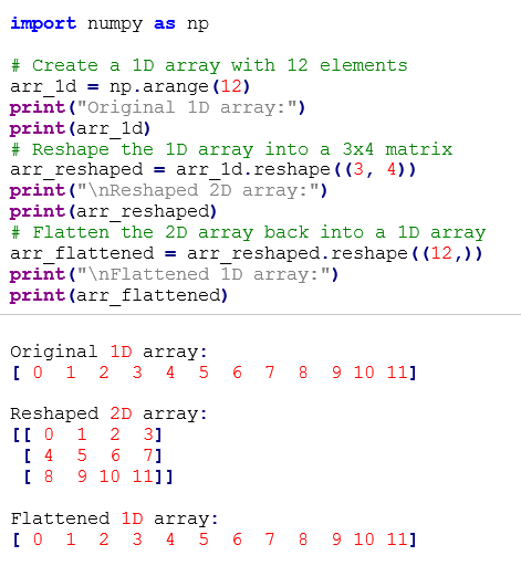
• We first create a 1D array which is ‘arr_1d’ it has 12 elements which we add using ‘np.arange(12)’.
• We then reshape the ‘arr_1d’ into a 3x4 matrix using ‘arr_reshape’ using ‘arr_1d.reshape((3, 4))’.
• Finally, we flatten ‘arr_reshaped’ back into a 1D array ‘arr_flattened’ using ‘arr_reshaped.reshape((12, ))’.

The above code demonstrates how ‘arr.reshape()’ can be used to change the shape of arrays while preserving their data.

Image source original

In NumPy, ‘arr.transpose()’ and ‘arr.T()’ are both used to transpose multi-dimensional arrays, effectively swapping their rows and columns. Here’s an explanation of each:

arr.transpose():

• The arr.transpose() method returns the array view with permuted axes. We may set the axis order using the axes option.
• Without a parameter, axes are rearranged. This is like flipping 2D array rows and columns.
• We use dot notation to call this array object function.

arr.T():

• The arr.T attribute transposes the array. It functions similarly to arr.transpose().
• It simplifies transpose array abbreviation, especially for brief code or interactive sessions.
• As an attribute, we access it directly from the array object without parenthesis.

Let’s look at the code for a better understanding of both arr.transpose() and arr.T().

This example shows that arr.transpose() and arr.T produce the identical transpose of the original array arr. This explains how to transpose multi-dimensional arrays in NumPy using both approaches.

Image source original

How to reverse an array

Learn about np.flip() with 1D, 2D, and multidimensional arrays in this section.

NumPy's np.flip() method reverses an array's contents along an axis. If we want to invert the array, we must provide the axis and array. NumPy reverses all input array axes if we don't specify the axis.

Using np.flip(), you may reverse array items along defined axes in NumPy. It manipulates arrays well and is used for data processing and analysis. This is a detailed explanation of np.flip(): 

• The input array is m, and the function syntax is np.flip(m, axis=None). An optional axis tuple or list of integers specifies the axes for component reversal. When not given, all axes are flipped.
• In the absence of an axis parameter, np.flip() flips the order of entries along all array axes. The axis parameter selects which axes are flipped. This lets us change dimensions while keeping others the same.
• Behavior Flipping: When np.flip() reverses the order of items along an axis, other axes stay fixed.Array flipping reverses item order in 1D. A 2D array reverses row order by flipping along the rows (axis=0) and column order by flipping along the columns (axis=1). We can flip multi-dimensional array members along a designated axis.
• Efficiency of Memory: Input array items are flipped along the given axes via np.flip(). It doesn't replicate the array, making it memory-efficient for large arrays.
• Applications: Image processing, signal processing, time series analysis, and data manipulation applications use np.flip() to flip images vertically or horizontally, reorder arrays for specific analyses, and reverse data sample order.

Finally, NumPy's np.flip() method gives several options for reversing element order along array axes. It is essential to various data processing operations and array manipulation.

Flipping a 1D array reverses element order. Specifying ‘axis=0’ flips a 1D array horizontally.

In a 2D array, we may flip items vertically or horizontally. Flipping rows and columns change their order.

Multi-dimensional array flipping: In a 2D array, we may flip items vertically or horizontally. Flipping rows and columns change their order.

Finally, the np.flip() method may reverse element order along selected axes in arrays of arbitrary dimension. It aids array transformations, image processing, and data manipulation.

Reshaping and flattening multidimensional arrays

This section covers.flatten() and.ravel().

Flattening an array usually involves.flatten() and.ravel(). The ravel() new array is a reference to the parent array, or "view," which is the key difference. This means that new array changes affect the parent array. Ravel utilizes less memory by not copying.

Flattening multi-dimensional arrays in NumPy creates a 1D array. This means the array's contents are in a linear sequence in their original order. Flatten() is explained in detail with an example of code:

• Method syntax: ‘array.flatten(order=’C’)’ flattens the multi-dimensional array ‘array’. ‘order’ (optional) determines element flattening order. The default is row-major (C-style) flattening (‘C’). For column-major (Fortran-style) flattening, use ‘F’.
• Flattening Applying ‘.flatten()’ to a multi-dimensional array flattens multidimensional array into a 1D array which is in a row-major order (by default). For example, ‘.flatten()’ will flatten a 2D array (2, 3) into a 1D array of length 6, in which row is in major order.
• Memory efficiency: unlike ‘.reshape()’, ‘.flatten()’ returns a duplicate of the flattened array, preserving the original array. This makes ‘.flatten()’ memory-efficient, especially for huge arrays, by not changing the original array.

Let’s see the Python code for a better understanding:

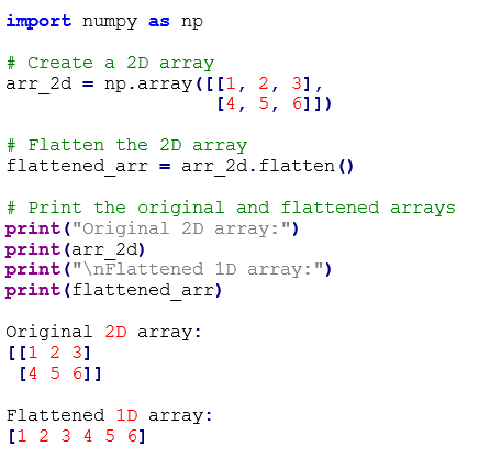
The preceding code creates a 2D array named ‘arr_2d’. We flatten ‘arr_2d’ with ‘.flatten()’ to create ‘flattened_arr’, a 1D array. Finally, we compare the original 2D and flattened 1D arrays by printing them.

In conclusion, the NumPy's.flatten() method helps convert multi-dimensional arrays to one-dimensional arrays while preserving elemental order. A flattened array duplicate is returned, making it useful for data processing and memory efficiency.

.ravel(): The NumPy.ravel() technique flattens multi-dimensional arrays into 1D arrays like.flatten(). However, the methods differ slightly. A detailed definition and code example of.ravel() are here:

• Method Syntax: ‘.ravel()’ syntax: array.ravel(order=’C’), where ‘array’ is the multi-dimensional array to flatten. ‘order’ (optional) determines element flattening order. The default is row-major (C-style) flattening (‘C’). For column-major (fortran-style) flattening, use ‘F’.
• Flattening Behavior: Same as ‘.flatten()’, ‘.ravel()’ flattens multi-dimensional arrays into 1D arrays. It traverses the array in row-major order (by default) and produces a 1D array with the contents in the same order as the multi-dimensional array. Instead of copying data, ‘.ravel()’ flattens the array wherever feasible. This improves memory efficiency, especially for big arrays.
• Memory Efficiency: ‘.ravel()’ returns the original array view whenever feasible, avoiding data duplication. This improves memory efficiency, especially for big arrays. If altering the flattened array may harm the original array, NumPy will duplicate the data to maintain data integrity.

Let’s look at the Python code for a better understanding:

The preceding code creates a 2D array named ‘arr_2d’. After applying ‘.ravel()’ on ‘arr_2d’, ‘flattened_arr’ is a 1D array. Finally, we compare the original 2D and flattened 1D arrays by printing them.

Finally, numpy.ravel() can transform multidimensional arrays into one-dimensional arrays while preserving elemental order. It utilizes little resources and returns a view of the original array wherever feasible, making it useful for many data transformation activities.

How to access the docstring for more information

In this section, we learn about help(), ?, ??.

Python and NumPy prioritize users in data science. Integration of documentation is a good example. Every object has a string reference called a docstring. Usually, this docstring comprises a brief object description and an example of use. Python's built-in help() function provides this information. This means we can utilize help() to discover information practically anytime.

Python's built-in help() function provides information on objects, modules, functions, classes, and methods. How to use Python components is also important, especially with libraries like NumPy, which have many methods and classes to explore.

Code sample and full explanation of ‘help()’:

Function syntax: ‘help()’ is simple. Pass the object or function we want information on as an argument. Without parameters, ‘help()’ opens an interactive help session where we may browse and search for information.

You may use ‘help()’ to acquire information on built-in objects, functions, classes, modules, or user-defined objects. When we send an object to ‘help()’, it shows its docstring, which describes its purpose, usage, arguments, return values, and examples. ‘help()’ provides object type and attribute information if there is no docstring.

When we supply the name of a module or function to ‘help()’, it shows its docstring and information about its classes, functions, and attributes. This clarifies the module or function's purpose and how to utilize it in our code.

To conclude, help() helps you understand and use Python modules, classes, methods, and objects. It provides detailed documentation to help you use Python components efficiently.

Use the?? and? symbols in specified contexts or libraries to access Python source code and documentation. They let users quickly discover functions, classes, modules, and objects without searching source files or external documentation.

‘?’ Question Mark: In IPython, Jupyter Notebooks, and certain IDEs, typing? followed by the name of an object, function, class, or module and executing the cell or command displays a brief description or docstring. Most descriptions include the object's usage, parameters, return values, and examples. Without having to leave our development environment, we can obtain documentation quickly.

‘??’ Double question marks: Similar to? in various Python environments,?? displays the object, function, class, or module's source code for further information. ?? displays the source code and docstring if available. This lets us see the logic and implementation details, which can help us understand how a function or method is implemented inside. However,?? may not work if the object is implemented in C or another compiled language or if the source code is unavailable.

Here’s an example demonstrating the use of ‘?’ and ‘??’ in IPython or Jupyter environment:

Should the aforementioned object be compiled in a language other than Python, utilizing?? will yield identical results to? This can be found in many pre-built objects and types, such as: 

Working with mathematical formulas

NumPy's simplicity of use for array mathematical formulae makes it popular in scientific Python. NumPy's formula editor rapidly computes and manipulates mathematical expressions, functions, and operations. NumPy's wide collection of mathematical functions and procedures for numerical arrays makes complex mathematical calculations easy. How to use NumPy with mathematical formulas:

The NumPy library, usually called ‘np’, must be imported first.

Define math formulas: Use NumPy functions and operators to define mathematical formulae. NumPy offers arithmetic, trigonometric, logarithmic, exponential, statistical, and linear algebra functions for many tasks.

Apply NumPy Functions: NumPy routines help apply mathematical formulas to data arrays. NumPy methods work element-by-element, thus we can modify whole arrays without loops.

Let’s see some example code:

We use two NumPy arrays, x, and y, as input. We use NumPy methods like np.sum(), np.dot(), and np.sin() to determine the sum of squares, dot product, and sin values of x components. Finally, we print the computed results.

Implementing the above formula is simple and straightforward in NumPy:

error = (1/n) * np.sum(np.square(predictions - labels))

The fact that labels and predictions might have one or a thousand values is what makes this system so effective. That is all that is required of them.

It can be seen like this:

Image source original

The labels and prediction vectors each contain three values, thus n is three. After subtractions, vector values are squared. After that, NumPy sums the values to give you the forecast inaccuracy and model quality score.

Image source original

NumPy is appropriate for a wide range of scientific, engineering, and mathematical applications because it performs numerical computations with mathematical formulae efficiently.

How to save and load NumPy objects

In this section, we will learn about np.save, np.savez, np.savetxt, np.load, and np.loadtxt.

Eventually, we'll need to load your arrays onto disk without rerunning the function. Thank goodness NumPy provides several save/load methods. The ndarray objects may be saved to and loaded from disk files using the loadtxt and savetxt procedures for standard text files, the load and save functions for NumPy binary files with a.npy extension, and the savez function for.npz files.

The data, shape, dtype, and other information needed to recreate the ndarray are kept in the.npy and.npz files, even on a different machine with a different architecture. This guarantees array retrieval.

np.save() saves a single ndarray object as an a.npy file. For many ndarray objects in one file, use np.savez to save them as.npz files. With savez_compressed, you may compress several arrays into one npz file.

Saving and loading an array with np.save() is easy. Include the file name and array we want to save.

NumPy's np.save() method saves arrays as ".npy" binary files. This method stores NumPy arrays efficiently and compactly on disk while preserving data types and forms. It's useful for storing large arrays like datasets, simulation results, and model parameters for sharing or use.

Example of np.save() with code:

Function syntax: ‘np.save()’ (file, arr). The array will be stored in a ‘file’ (with the location if required). We wish to store the NumPy array ‘arr’.

Save NumPy arrays: A NumPy array and a file name are sent to ‘np.save()’ to build a binary file and store the array contents. The stored file contains the binary array data and metadata such as data type, shape, and other information needed to reassemble it.

Example code:

Loading Saved Arrays: we can later load the saved array back into memory using the ‘np.load()’ function. for example, to load the array saved in the previous example:

Finally, NumPy's np.save() method is handy for disk-based binary array storage. It's easy to save and retrieve NumPy arrays, making it useful for sharing and storing data in scientific and numerical computing applications.

np.savez(): NumPy's np.savez() method may merge many arrays into a ".npz" archive. This function compresses and stores several arrays in one file, making it useful for sharing datasets, models, and experiment results.

With an example code, ‘np.savez()’ works:

Functional syntax: ‘np.savez()’ is ‘np.savez(file, *args, **kwds)’, where ‘file’ is the file name (with the path if required) where the arrays will be stored. NumPy arrays ‘*args’ should be saved. Arguments can be several arrays. The optional keywords ‘**kwds’ allow array names and other customization.

Using ‘np.savez()’ with a file name and one or more NumPy arrays generates a “.npz” archive file and saves the arrays. The stored file comprises compressed binary array representations and metadata like data type, shapes, and other information needed to rebuild them.

An example code: Sample code using ‘np.savez()’ to save multiple arrays: 

Later, we may use ‘np.load()’ to load stored arrays into memory. example: loading the arrays saved in the previous example:

Finally, NumPy's np.savez() method may compress several arrays into one file. Since it stores and retrieves multiple arrays efficiently, it is useful for data exchange and storage in scientific and numerical computing applications.

np.savetxt(): NumPy's np.savetxt() method saves arrays to text. This method lets us export NumPy array data to plain text files that other users and apps may access.

Check out ‘np.savetxt()’ with an example:

This function uses the syntax ‘np.savetxt(fname, X, fmt=’%.18e’, delimiter=‘ ‘, newline=‘\n’, header=‘ ‘, footer=‘ ‘, comments=‘# ‘, encoding=None)’. The array will be stored to ‘fname’, providing the path if needed. We wish to store NumPy array ‘X’. Text file numbers are formatted using ‘fmt’. The default is ‘%.18e’ (scientific notation with 18 decimal digits). The string ‘delimiter’ separates text file values. Space is the default. The string ‘newline’ ends each text file line. The Newline character ‘\n’ is the default. A string called ‘header’ will start the file. Files conclude with a string called ‘footer’. The string ‘comments’ will indicate file comments. # (hash + space) defaults. File encoding is called ‘encoding’. System default encoding is None.

Save Array as Text: Using np.savetxt() with a NumPy array and file name creates a text file and saves the array contents. Each member of the array is formatted as text in the stored file using the format string and delimiter.

Example code: ‘np.savetxt()’ saves a NumPy array to a text file: 

The preceding code creates a 2D NumPy array ‘arr’. We use ‘np.savetxt()’ to save the array to ‘my_array.txt’ with the format string as “%d” (integer) and the delimiter as ‘,’. After that, we print a message confirming the array saving to the text file. We use ‘open()’ with “r” (read) mode to access “my_array.txt” after storing it. We then print a message indicating file printing. Lastly, we use “file.read()” to read and output the file contents to the console.

Using np.savetxt(), you may export array data to text files for analysis, visualization, or dissemination. It lets us customize the output text file's structure and format.

np.load() loads arrays or pickled objects from ".npy", ".npz", or pickled files in NumPy. This method restores binary or text NumPy arrays or objects.

See how ‘np.load()’ works with an example code:

Function syntax: ‘np.load(file, mmap_mode=None, allow_pickle=True, fix_imports=True, encoding=‘ASCII’)’, where ‘file’ is the name (with the path if required) of the array or object to be loaded. ‘mmap_mode’ controls data access via memory-mapped file objects. The default is None. ‘allow_pickle’ is a Boolean flag that allows pickled object loading. Defaults to True. ‘fix_imports’ is a Boolean flag that determines whether Python3 should fix Python 2 pickle files. Defaults to True. Text file loading uses ‘encoding’. Defaults to ‘ASCII’.

When we use ‘np.load()’ with the file name, it reads the data from the file and returns the array or object. Data is loaded automatically based on file format (“.npy”, “.npz”, or pickled).

Example code: ‘np.load()’ loads a NumPy array from a “.npy” file.

The preceding code loads a NumPy array from “my_array.npy” using ‘np.load()’. The variable ‘loaded_array’ stores the loaded array. Printing the loaded array verifies that I was loaded from the file.

The useful np.load() function loads and stores NumPy arrays and objects. Data can be processed, analyzed, or displayed in Python programs. Its easy-to-access data makes it valuable in scientific, engineering, and numerical computer applications.

np.loadtxt(): NumPy arrays may load text file data using np.loadtxt(). This function converts numerical data from plain text files into NumPy arrays for processing, analysis, and presentation.

See how ‘np.loadtxt()’ works with an example code:

Function Syntax: 'np.loadtxt(fname, dtype=float, comments=‘#’, delimiter = None, converters = None, skiprows=0, usecols=None, unpack=False, ndim=0, encoding=’bytes’, max_rows=None)', where 'fname' is the file name (including the path if necessary) from which data will be loaded. 'dtype' indicates the array's data type. The default is float. 'comments' indicates file comments. Comment-starting lines are disregarded. Defaults to '#'. The string 'delimiter' separates file values. The default is None, meaning whitespace. 'converters' is a dictionary that maps column numbers or names to functions that convert string values to data types. To skip, enter'skiprows' rows at the beginning of the file. Defaults to 0. The sequence of column indices or names 'usecols' specifies which file columns to read. Transpose of the loaded array using the Boolean flag 'unpack'. The default is False. The array should have at least 'ndmin' dimensions. Defaults to 0. Text file loading uses 'encoding'. The default is 'bytes'. File reading is limited to'max_rows'. The default is None, reading all rows.

Loading Data from Text File: When we use ‘np.loadtxt()’ with the file name, it reads the numerical data and turns it into a NumPy array. The function automatically recognizes the text file's delimiter and data types and turns the contents into an array.

An example code: This code shows how to use ‘np.loadtxt()’ to load numerical data from a text file:

We build a 5x3 array of integers between 0 and 100 using ‘np.random.randint()’ in the preceding code. The resulting numerical data is stored to “my_data.txt” using ‘np.savetxt()’. To separate values with commas, we use ‘,’. Next, we use ‘np.loadtxt()’ to load numerical data from “my_data.txt” into a NumPy array. To properly parse data, we use ‘,’ again. Finally, we print the loaded data to confirm loading. The text file data array is printed.

Using np.loadtxt(), we can easily load numerical data from text files or other datasets into our Python scripts. It is flexible enough to import data from several file formats and alternatives for research, engineering, and data analysis applications.

Summary

NumPy, a Python numerical computing staple, offers a large toolbox for arrays and matrices. The flexible ndarray data structure works with matrices and multi-dimensional arrays. These arrays can effectively store and analyze large volumes of numerical data, enabling many scientific computing and data analysis activities.

The library has several array generate and initialize methods, from fundamental constructors like np.array() to more specialized ones like np.zeros(), np.ones(), np.arange(), and np.random.randint(). These diverse array-building tools allow users to easily generate arrays for modeling, simulation, or data representation.

One of NumPy's most significant features is precise indexing and slicing for array manipulation. NumPy has several techniques for manipulating and examining array contents, including basic indexing, axes-based slicing, and Boolean mask selection.

NumPy simplifies element-wise operations like addition, subtraction, multiplication, and division with its powerful array operator suite. Broadcasting allows NumPy to compute smoothly over arrays of different widths and shapes.

NumPy's data aggregation and reduction capabilities, such as np.sum(), np.mean(), np.max(), and np.min(), simplify statistics and array data summarization along defined axes. These routines provide valuable insights from complex datasets.

NumPy can concatenate, divide, stack, and flatten arrays for many array manipulation needs. These tools let users effortlessly restructure and transform array data for seamless inclusion into analytical workflows.

NumPy prioritizes economy and performance with its optimized C and Fortran code for lightning-fast processing. NumPy is best for sophisticated numerical calculations and scientific library integration due to its performance.

To conclude, NumPy is crucial for numerical simulations, data analysis, and scientific computing in Python. It is preferred by enthusiasts and specialists who wish to tackle complex numerical problems quickly and efficiently due to its performance-oriented architecture and excellent array manipulation capabilities.